SnappyHexMesh Tutorial: Patient-Specific Aorta Meshing

Overview

This comprehensive tutorial covers advanced techniques for creating high-quality computational meshes for patient-specific aorta geometries using OpenFOAM's snappyHexMesh utility. Learn the complete workflow from STL preparation to simulation-ready mesh generation with physiologically accurate boundary conditions.

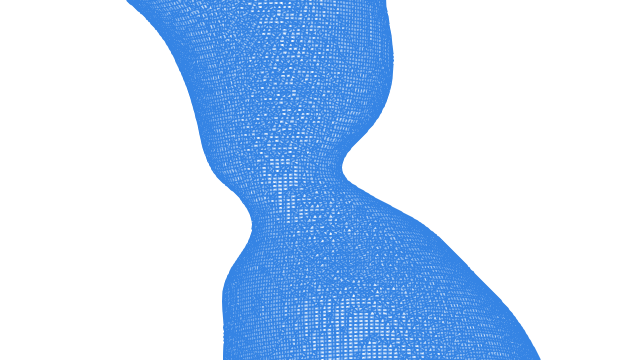Patient-specific aorta mesh generated with snappyHexMesh, showing refined boundary layers and branch resolution.

Prerequisites

Required Knowledge & Tools

• OpenFOAM: Version 12 (Foundation) installed and configured
• Basic CFD Understanding: Familiarity with mesh generation concepts
• Linux/Unix: Command line proficiency
• Geometry Files: Patient-specific STL files prepared

Understanding Aorta Geometry

The aorta presents unique meshing challenges that require specialized techniques:

Key Geometric Challenges

• 🫀 Complex Bifurcations: Aortic arch branches require careful feature edge detection and local refinement
• 📏 Variable Diameter: From ascending (≈30mm) to small branches (≈5mm) - automatic refinement essential
• 🌊 Curved Geometry: Sharp curvatures need proper cell aspect ratios and orthogonality
• 🌳 Branch Vessels: Small outlets require adequate cross-sectional resolution (>10 cells)

Required Input Files

case/constant/triSurface/
├── wall_aorta.stl      # Main vessel wall
├── inlet.stl           # Inlet boundary  
├── outlet_desc.stl     # Descending aorta outlet
├── outlet_bca.stl      # Brachiocephalic outlet
├── outlet_lcca.stl     # Left common carotid
└── outlet_lsca.stl     # Left subclavian

Background Mesh Setup

The background mesh defines your computational domain and must encompass the entire aorta geometry with appropriate margins.

blockMeshDict Configuration

FoamFile
{
    version     2.0;
    format      ascii;
    class       dictionary;
    object      blockMeshDict;
}

convertToMeters 1;

vertices
(
    (-0.1 -0.1 -0.1)    // Minimum bounding box
    ( 0.1 -0.1 -0.1)
    ( 0.1  0.1 -0.1)
    (-0.1  0.1 -0.1)
    (-0.1 -0.1  0.3)    // Maximum bounding box
    ( 0.1 -0.1  0.3)
    ( 0.1  0.1  0.3)
    (-0.1  0.1  0.3)
);

blocks
(
    hex (0 1 2 3 4 5 6 7) (40 40 80) simpleGrading (1 1 1)
);

Domain Sizing Guidelines

• Margins: 5-10 vessel diameters from geometry surface
• Aspect Ratio: Keep background cells roughly cubic
• Resolution: Start with 1-2mm cell size for typical aorta

Feature Edge Detection

Feature edges are critical for capturing vessel bifurcations and ensuring proper mesh topology at complex junctions.

Extract Features

# Extract feature edges from STL surfaces
surfaceFeatureExtract -includedAngle 150

This creates .eMesh files containing feature edge information.

snappyHexMeshDict Configuration

castellatedMeshControls
{
    features
    (
        {
            file "wall_aorta.eMesh";
            level 2;        // Refinement at feature edges
        }
    );

    resolveFeatureAngle 30;     // Detect features > 30°
    planarAngle 30;             // Planar surface angle
}

Why Feature Detection Matters

• Bifurcation Capture: Ensures branch junctions are properly resolved
• Geometry Fidelity: Maintains sharp edges and transitions
• Mesh Quality: Prevents poor cells at geometric features
• Flow Physics: Accurate representation affects hemodynamics

Common Issue

If resolveFeatureAngle is too small (< 20°), you may get excessive refinement and poor mesh quality.

Geometric Alignment: Critical for Mesh Quality

Proper geometric alignment with the coordinate system is crucial for snappyHexMesh quality. Research from PhD studies demonstrates that misaligned geometries lead to significantly degraded mesh quality and numerical instability.

Impact of Geometric Misalignment

A systematic study using U-bend geometries with progressive 45-degree rotations (XY, XZ, YZ planes) demonstrated that misalignment with the background mesh coordinate system degrades mesh quality significantly:

Configuration	Max Non-Orthogonality	Max Skewness	Boundary Layer Coverage
Aligned (original)	~45 deg	~1.5	>95%
XY rotation (45 deg)	~55 deg	~2.5	~85%
XY+XZ rotation	~65 deg	~3.5	~75%
XY+XZ+YZ rotation	~70 deg	~4.0	~65%

These results indicate that misaligned geometries produce higher skewness and non-orthogonality, distorted boundary layers, and degraded near-wall cell quality that directly affects hemodynamic predictions such as wall shear stress Jasak 1996.

Automated Alignment in AortaCFD

PCA-Based Alignment in AortaCFD

AortaCFD automatically aligns patient geometries using Principal Component Analysis (PCA). The algorithm extracts surface vertices from the combined STL patches, computes the three principal axes via eigendecomposition of the covariance matrix, and applies a rotation matrix to align the geometry's longest axis with the Z-coordinate. This is implemented in src/aortacfd_lib/aorticAxisEstimator.py.

Alignment Best Practices

Manual Alignment Guidelines

If not using automated tools:

1. Orient longest axis along Z-coordinate (flow direction)
2. Center geometry at coordinate origin
3. Minimize rotations from principal axes
4. Check bounding box alignment with coordinate planes
5. Verify inlet/outlet normal vectors align with coordinate axes

Quality Metrics Improvement

Proper alignment typically improves: - Non-orthogonality: 30-50% reduction in maximum values - Skewness: 40-60% improvement in boundary cells - Boundary layers: More uniform thickness distribution - Convergence: Faster solver convergence and stability

Surface Refinement Strategy

Different regions of the aorta require different mesh densities based on flow physics and geometric complexity.

refinementSurfaces Configuration

refinementSurfaces
{
    wall_aorta
    {
        level (1 2);        // Base refinement: 1-2 levels

        regions
        {
            // Localized refinement for critical areas
            arch
            {
                level (2 3);    // Higher at aortic arch
            }
            branches
            {
                level (3 4);    // Highest at bifurcations
            }
            stenosis
            {
                level (4 5);    // Maximum for pathology
            }
        }
    }

    inlet
    {
        level (2 3);           // High refinement for inlet profile
        patchInfo
        {
            type patch;
        }
    }

    "outlet.*"
    {
        level (2 3);           // Adequate outlet resolution
        patchInfo
        {
            type patch;
        }
    }
}

Automatic Refinement Levels

AortaCFD Automatic Calculation

AortaCFD automatically calculates optimal refinement levels based on minimum vessel diameter:

Quality Level	Cells per Diameter	Cell Size	Use Case
Coarse	10-12 cells/D	200k-500k cells	Geometry checks, initial exploration
Standard	15-20 cells/D	500k-2M cells	Production simulations (recommended)
Fine	25-30 cells/D	2M-5M cells	Mesh independence studies

Resolution is controlled by the cells_per_diameter parameter in config.json. Cell counts vary with anatomy.

Global Refinement Strategy

Based on PhD research, AortaCFD employs a global refinement approach that provides several advantages over local refinement strategies:

Global vs. Local Refinement

Global Refinement Benefits: - Uniformly high resolution throughout the domain - Simplified user experience - no complex region definitions - LES compatibility - consistent resolution for turbulence modeling - Flexible resource scaling - easy adjustment for computational constraints

Why Global Refinement was Chosen: - Early development tested "searchableBox" local refinement - Added complexity with limited flexibility across patient geometries - Global approach achieves sufficient control while maintaining simplicity - Better suited for automated workflows and batch processing

Research-Validated Quality Targets

Based on extensive cardiovascular CFD research, the following quality thresholds are recommended:

Mesh Quality Targets for Cardiovascular CFD

Metric	Target Range	Clinical Impact
Non-orthogonality	< 60° (max 70°)	Affects pressure gradient accuracy
Skewness	< 1.5 internal, < 4 boundary	Critical for wall shear stress
Cell volume ratio	> 0.01	Prevents convergence issues
Aspect ratio	< 100 near walls	Important for boundary layer resolution
Y+ values	< 1 (wall-resolved)	Required for accurate WSS calculation

Span-Based Refinement

For stenotic or coarctation cases, span-based refinement ensures adequate cross-sectional resolution.

Configuration for Stenosis

refinementRegions
{
    wall_aorta
    {
        mode            insideSpan;
        level           (1000 3);       // Distance and refinement level
        cellsAcrossSpan 30;             // Minimum cells across diameter
    }

    // Alternative: distance-based refinement
    stenosis_region
    {
        mode            inside;
        level           4;

        // Define region geometry
        cylinder
        {
            point1 (0.02 0.01 0.15);    // Start point
            point2 (0.02 0.01 0.20);    // End point  
            radius 0.015;                // Refinement radius
        }
    }
}

Stenosis Refinement Guidelines

Severity	Diameter Reduction	Cells Across	Reasoning
Mild	< 30%	20 cells	Capture basic flow disturbance
Moderate	30-50%	30 cells	Resolve recirculation zones
Severe	> 50%	40 cells	Capture jet formation/breakdown

Boundary Layer Generation

Accurate wall shear stress calculation requires proper near-wall mesh resolution through prismatic boundary layers.

addLayersControls Configuration

addLayersControls
{
    relativeSizes       true;           // Use relative sizing

    layers
    {
        wall_aorta
        {
            nSurfaceLayers 5;           // 5 prismatic layers
        }
    }

    expansionRatio      1.2;            // Layer growth ratio
    finalLayerThickness 0.3;            // 30% of surface cell size
    minThickness        0.1;            // Minimum absolute thickness

    // Quality controls
    featureAngle        60;             // Layer collision angle
    slipFeatureAngle    30;             // Allow slip at features
    nRelaxIter          5;              // Relaxation iterations
    nSmoothSurfaceNormals 1;            // Surface normal smoothing
    nSmoothNormals      1;              // Volume normal smoothing
    nSmoothThickness    10;             // Thickness field smoothing

    // Advanced controls
    maxFaceThicknessRatio 0.5;          // Face thickness ratio
    maxThicknessToMedialRatio 0.3;      // Medial axis ratio
    minMedianAxisAngle  90;             // Medial axis angle
    nBufferCellsNoExtrude 0;            // Buffer zone
    nLayerIter          50;             // Maximum iterations
}

Y+ Targeting

Y+ Requirements for Cardiovascular Flows

• y+ < 1: Wall-resolved simulation (DNS/LES)
• y+ = 30-300: Wall function approach (RANS)
• Avoid: 5 < y+ < 30 (buffer region)

\[y^+ = \frac{u_\tau y}{\nu}\]

Where \(u_\tau\) is friction velocity, \(y\) is wall distance, \(\nu\) is kinematic viscosity.

Layer Thickness Calculation

For y+ ≈ 1 in aortic flow:

# Estimate first layer thickness
Re = 4000          # Typical aortic Reynolds number
D = 0.025          # Vessel diameter (m)
nu = 1.5e-6        # Blood kinematic viscosity at 37°C

# Wall shear stress estimation
tau_w = 0.5 * rho * U^2 * f/8  # Empirical correlation
u_tau = sqrt(tau_w / rho)      # Friction velocity

# First layer thickness for y+ = 1
delta_1 = nu / u_tau  # ≈ 20-50 μm

Common Layer Issues

• Collision at bifurcations: Reduce finalLayerThickness or featureAngle
• Poor coverage: Increase nRelaxIter and smoothing parameters
• Excessive skewness: Check surface mesh quality first

Mesh Quality Controls

Robust quality controls ensure numerical stability and accuracy of CFD simulations.

meshQualityControls Configuration

meshQualityControls
{
    // Primary quality metrics
    maxNonOrtho         65;         // Non-orthogonality limit
    maxBoundarySkewness 20;         // Boundary skewness
    maxInternalSkewness 4;          // Internal skewness
    maxConcave          80;         // Concavity angle

    // Volume and area constraints
    minVol              1e-13;      // Minimum cell volume
    minTetQuality       1e-30;      // Tetrahedral quality
    minArea             -1;         // Minimum face area (disabled)
    minTwist            0.02;       // Face twist factor
    minDeterminant      0.001;      // Mesh determinant
    minFaceWeight       0.05;       // Face interpolation weight
    minVolRatio         0.01;       // Adjacent cell volume ratio

    // Smoothing and error reduction
    nSmoothScale        4;          // Smoothing iterations
    errorReduction      0.75;       // Error reduction factor

    // Relaxed quality during mesh generation
    relaxed
    {
        maxNonOrtho     75;
        maxBoundarySkewness 25;
        maxInternalSkewness 8;
    }
}

Quality Verification

# Comprehensive mesh check
checkMesh -allGeometry -allTopology

# Key metrics to verify:
# ✓ Non-orthogonality < 70°
# ✓ Skewness < 4
# ✓ Aspect ratio < 100
# ✓ All cells positive volume

Expected Quality Ranges

Metric	Excellent	Good	Acceptable	Poor
Non-orthogonality	< 45°	< 65°	< 75°	> 75°
Skewness	< 1	< 2	< 4	> 4
Aspect Ratio	< 10	< 50	< 100	> 100

Running snappyHexMesh

Execute the mesh generation process with proper monitoring and parallel efficiency.

Sequential Execution

# Step 1: Create background mesh
blockMesh

# Step 2: Extract feature edges  
surfaceFeatureExtract

# Step 3: Run snappyHexMesh
snappyHexMesh -overwrite

# Step 4: Check mesh quality
checkMesh -allGeometry -allTopology

Parallel Execution

# Decompose domain for parallel processing
decomposePar -noZero -force

# Run snappyHexMesh in parallel
mpirun -np 8 snappyHexMesh -parallel -overwrite

# Reconstruct the mesh
reconstructParMesh -constant -latestTime

# Clean up processor directories
rm -rf processor*

# Final quality check
checkMesh -allGeometry -allTopology

AortaCFD Automated Parallel Processing

AortaCFD implements intelligent parallel processing based on research optimisation:

# Research-based parallel automation from PhD thesis
def run_parallel_meshing(n_processors, case_dir):
    """
    Automated parallel snappyHexMesh execution with optimization
    """
    if parallel_meshing_enabled:
        # Decompose for parallel processing
        os.system("decomposePar -noZero -force")

        # Execute snappyHexMesh in parallel
        cmd = f"mpirun -np {n_processors} snappyHexMesh -parallel -overwrite"
        os.system(cmd)

        # Reconstruct mesh
        os.system("reconstructParMesh -constant -latestTime")

        # Clean up processor directories
        os.system("rm -rf processor*")
    else:
        # Sequential execution for small cases
        os.system("snappyHexMesh -overwrite")

Performance Optimization

Resource Requirements

Recommended Core Counts: - Small mesh (< 2M cells): 4-8 cores - Medium mesh (2-8M cells): 8-16 cores
- Large mesh (> 8M cells): 16-32 cores

Memory Requirements: - Estimate 1-2 GB RAM per million cells - Add extra for feature extraction and layer addition

Expected Mesh Statistics

Quality	Cell Count	Generation Time	Memory Usage
Coarse	1-2M	10-30 min	4-8 GB
Medium	3-5M	30-90 min	8-16 GB
Fine	8-12M	2-4 hours	16-32 GB

Next Step: Boundary Conditions

Once your mesh is generated and validated, the next critical step is setting up physiologically accurate boundary conditions.

Boundary Conditions Tutorial

📖 Boundary Conditions for Cardiovascular CFD

This comprehensive tutorial covers: - Inlet conditions: Pulsatile flow profiles and patient-specific data - Outlet modeling: 3-element Windkessel and advanced pressure models
- Wall boundaries: Rigid and moving wall implementations - Physiological parameters: Age-adjusted values and validation targets - Integration: Complete case setup and solver compatibility

Validation and Results

Mesh Validation

# Final comprehensive check
checkMesh -allGeometry -allTopology -constant

# Mesh statistics
foamLog log.snappyHexMesh

# ParaView visualization
paraFoam

Key Validation Points

• ✅ All quality metrics pass
• ✅ Boundary layer coverage > 90%
• ✅ Feature edges properly captured
• ✅ No negative volume cells
• ✅ Smooth refinement transitions

Expected Flow Physics

The mesh should resolve:

• Dean vortices in curved sections
• Recirculation zones at bifurcations
• Wall shear stress gradients
• Pressure drop across stenosis
• Transitional flow features

Quality Indicators

• y+ values in target range
• Convergent residuals (< 1e-6)
• Reasonable pressure gradients
• Physiological wall shear stress (0.5-2.5 Pa)

Integration with AortaCFD

Automated Mesh Generation in AortaCFD

The entire process is automated in the AortaCFD pipeline:

# Complete mesh generation
python run_patient.py BPM120 --steps case,mesh

# With specific resolution
python run_patient.py BPM120 --steps case,mesh --config config_mesh_fine.json

Automated features include PCA-based geometry alignment, global refinement controlled by cells_per_diameter, parallel snappyHexMesh execution, mesh quality assessment with adaptive numerics via the regenerate-numerics step, and quality reporting.

Automation Workflow

The AortaCFD pipeline automates each stage of mesh generation based on validated research methodologies:

Step	Manual Process	AortaCFD Automation
Geometry Prep	Manual alignment, unit conversion	PCA alignment, auto-scaling from STL
Mesh Setup	Complex snappyHexMeshDict editing	Template-based generation from cells_per_diameter
Quality Control	Manual checkMesh interpretation	Automated quality assessment and adaptive numerics
Parallel Execution	Manual decomposition/reconstruction	Configured via run_settings.subdomains
Validation	Manual mesh inspection	Automated quality reporting to reports/

Quick Reference

Key Takeaways

• Feature edges are essential for bifurcation capture
• Span refinement ensures adequate cross-sectional resolution
• Boundary layers are critical for wall shear stress accuracy
• Quality control prevents numerical instabilities
• Physiological BCs are required for meaningful results

References

Full bibliography on the References page.

Next Steps

• Windkessel Tutorial - 3-Element RCR boundary conditions
• GitHub Repository - Complete automated workflow
• OpenFOAM Documentation - Official OpenFOAM guides

Found an issue or have a suggestion for this page?

Open a GitHub issue