Tutorial 2: Inlet and Outlet Conditions
Goal: Understand how AortaCFD handles physiological boundary conditions -- pulsatile inlets and Windkessel outlets.
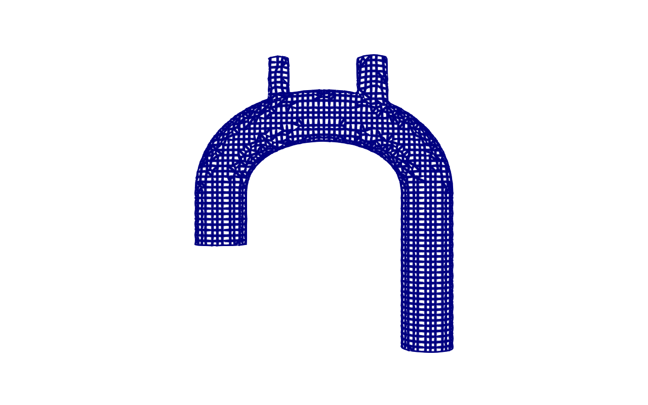 Branched tube with 3 outlets used in this tutorial. You will learn how Windkessel boundary conditions model the downstream vasculature and how pulsatile inlet waveforms drive the cardiac cycle.
Hands-On Exercise
Download: exercise_06_windkessel.tar.gz (14 MB) | ~6 sec | OpenFOAM 12 + WKBC library
Branched tube with 3 outlets, pre-meshed. Includes pre-computed results showing Windkessel pressure response.
Introduction
Standard OpenFOAM tutorials typically use fixed-pressure or zeroGradient outlet conditions, which are adequate for steady industrial flows. In cardiovascular CFD, the boundary conditions must reflect the physiology of the cardiac cycle: a pulsatile inlet driven by the heart and outlet conditions that represent the resistance and compliance of the downstream vasculature.
This tutorial covers the inlet and outlet boundary condition types available in AortaCFD, explains the physical rationale for each, and demonstrates the Windkessel outlet model on a branched tube geometry.
By the end of this tutorial you will be able to:
- Select the appropriate inlet type based on available clinical data.
- Configure constant and time-varying inlet conditions.
- Explain the role of Windkessel outlet boundary conditions.
- Understand how Murray's law distributes resistance across outlets.
- Recognise why backflow stabilisation is necessary during diastole.
Why Boundary Conditions Matter
The cardiac cycle drives a periodic pressure and velocity waveform through the arterial system. During systole (~35% of the cycle), the left ventricle ejects blood into the aorta at peak velocities of 1--2 m/s. During diastole (~65% of the cycle), the aortic valve closes and flow decelerates; at outlet boundaries, flow may reverse temporarily.
The choice of boundary conditions directly governs:
- Pressure levels throughout the domain.
- Flow distribution between outlets (e.g., how much blood flows to each branch of the aortic arch versus the descending aorta).
- Solver stability during flow reversal phases.
- Clinical accuracy of computed wall shear stress and pressure gradients.
Fixed Pressure Is Not Physiological
Setting all outlets to a fixed pressure (e.g., fixedValue 0) forces
the pressure distribution to be determined entirely by the inlet condition
and the internal flow field. This eliminates the resistance and compliance
effects of the downstream vasculature and produces non-physiological flow
splits between branches.
Inlet Types
AortaCFD supports two primary inlet types, selected via the inlet.type
field in config.json.
CONSTANT Inlet
A constant inlet imposes a steady flow rate derived from the specified cardiac output (in L/min). AortaCFD computes the mean velocity from the inlet area:
| Advantage | Limitation |
|---|---|
| Simplest to configure | No pulsatility |
| No CSV file required | Cannot compute time-dependent metrics (OSI, RRT) |
| Good for pressure-drop estimation | WSS is time-averaged only |
When to Use CONSTANT
Use a constant inlet for quick feasibility tests, debugging mesh or solver issues, and computing steady-state pressure drops. It is not appropriate for studies reporting oscillatory shear index or any metric that depends on the temporal flow waveform.
TIMEVARYING Inlet
{
  "inlet": {
    "type": "TIMEVARYING",
    "csv_file": "flowrate.csv",
    "data_type": "flowrate",
    "profile": "parabolic"
  }
}
A time-varying inlet reads a pulsatile flow waveform from a CSV file. This is the standard inlet type for production cardiovascular CFD simulations.
CSV format:
| Column | Name | Units | Description |
|---|---|---|---|
| 1 | Time | s | Time within the cardiac cycle |
| 2 | Flowrate | m^3/s or L/min | Volumetric flow rate at each time point |
Example CSV content:
Automatic Unit Detection
AortaCFD inspects flow-rate magnitudes to infer units: values greater than 1 are treated as L/min; values on the order of 1e-5 are treated as m^3/s. The CSV is interpolated to the simulation time steps automatically.
Profile options: plug (uniform velocity), parabolic (Poiseuille-like),
wall_distance (distance-based, good for non-circular inlets), womersley
(analytical pulsatile solution).
Outlet Types
AortaCFD supports two outlet boundary condition types.
zeroGradient Outlet
The simplest outlet condition. It extrapolates the pressure field from the interior to the outlet face, imposing zero normal gradient. No downstream vascular resistance or compliance is modelled.
| Advantage | Limitation |
|---|---|
| No parameters to set | Non-physiological pressure levels |
| Never crashes from BC coupling | Incorrect flow splits between branches |
| Good for debugging | Not suitable for production runs |
3EWINDKESSEL Outlet
{
  "outlets": {
    "type": "3EWINDKESSEL",
    "enable_stabilization": true,
    "blood_pressure": { "systolic": 120, "diastolic": 80 }
  }
}
The 3-element Windkessel model (RCR) represents the downstream vasculature as an electrical analogue circuit with three components. Explore how each parameter affects the pressure waveform:
| Parameter | Symbol | Physical Meaning | Controls |
|---|---|---|---|
| Proximal resistance | R1 (or Z) | Resistance to pressure waves | Wave reflections |
| Compliance | C | Arterial wall distensibility | Pulse pressure amplitude |
| Distal resistance | R2 (or R) | Downstream vascular resistance | Mean pressure level |
The governing equation couples the outlet pressure to the instantaneous flow rate:
where the distal pressure \(P_d\) evolves according to:
Kinematic Units
OpenFOAM uses kinematic units (divided by density). All Windkessel
parameters in the 0/p file are in kinematic form. AortaCFD handles the
conversion automatically -- you specify blood pressure in mmHg in the
config, and the tool computes the kinematic R, C, and Z values.
Running the Exercise
Extract and Run
The exercise contains a branched tube geometry with one inlet and three outlets, pre-meshed and configured with Windkessel boundary conditions:
| Directory | Description |
|---|---|
case_with_stab/ |
Windkessel outlets with backflow stabilisation enabled |
precomputed/ |
Pre-computed results showing pressure waveforms |
Run the simulation:
The simulation completes in approximately 6 seconds. Examine the pressure boundary condition file:
You will see Windkessel parameters on each outlet patch:
These values are in kinematic units (m^2/s^2 for pressure, kinematic resistance, and kinematic compliance). AortaCFD computes them automatically from the specified blood pressure and outlet geometry.
Murray's Law and Resistance Distribution
When a geometry has multiple outlets, the total peripheral resistance must be distributed among them. AortaCFD uses Murray's law to perform this distribution automatically.
The Principle
Murray's law states that vascular resistance scales inversely with the cube of the vessel diameter:
For a geometry with \(N\) outlets, the resistance assigned to outlet \(i\) is:
This means:
- Larger outlets receive lower resistance (more flow).
- Smaller outlets receive higher resistance (less flow).
Physiological Basis
Murray's law arises from the principle of minimum work: the metabolic cost of maintaining blood (proportional to vessel volume) is balanced against the energy dissipated by viscous flow (proportional to resistance). The optimal vessel radius that minimises total biological cost obeys the cube-law relationship Murray 1926.
Practical Consequence
In an aortic geometry with four outlets, the descending aorta (largest diameter, ~20 mm) receives the lowest resistance and carries the majority of the cardiac output (~65--70%). The supra-aortic branches (8--12 mm each) receive proportionally higher resistance. This automatic distribution produces physiologically reasonable flow splits without manual tuning.
Examining the Distribution
After running a case with Windkessel outlets, AortaCFD reports the computed flow split in the simulation setup report:
Look for the outlet flow distribution table, which lists the resistance value, flow fraction, and mean pressure for each outlet.
Backflow Stabilisation
The Problem
During diastole, the decelerating and partially reversing flow creates regions where fluid enters the domain through outlet boundaries. Without stabilisation, this reversed flow carries unphysical velocity information into the domain, generating spurious vortices that can:
- Destabilise the pressure-velocity coupling.
- Cause the time step to collapse as the adaptive controller tries to maintain stability.
- Ultimately crash the solver.
The Solution
The modularWKPressure boundary condition in AortaCFD includes a backflow
stabilisation mechanism controlled by the betaT parameter:
| Parameter | Purpose | Recommended Value |
|---|---|---|
betaT |
Tangential velocity damping on reversed flow | 0.3 |
betaN |
Normal velocity damping on reversed flow | 0.0 |
When flow reverses at an outlet face, the stabilisation term damps the
tangential velocity component to suppress vortex formation. The normal
component (betaN) is left at zero to preserve the Windkessel
pressure-flow coupling.
Do Not Set betaN > 0 Unless Necessary
Setting betaN > 0 introduces a resistance-like term that modifies the
pressure-flow relationship of the Windkessel model. This can bias the
computed pressure waveform. Only increase betaN when severe diastolic
instabilities persist despite mesh refinement.
What Happens Without Stabilisation
If you run the same geometry without backflow stabilisation on a coarse mesh, you may observe:
- Rapidly collapsing time step during diastole.
- PIMPLE outer loop failing to converge.
- Floating-point exception or solver crash.
On finer meshes (cpd > 15 with boundary layers), the solver may survive without stabilisation, but enabling it provides a safety margin at negligible computational cost.
Exercise: Inspect the Windkessel Response
After running the exercise case, examine the pressure evolution at an outlet:
Or plot the pressure from the pre-computed results:
Observe the following features:
- Systolic peak: Pressure rises rapidly as flow accelerates.
- Diastolic decay: Pressure decays exponentially, governed by the RC time constant (\(\tau = R \cdot C\)).
- Phase lag: The Windkessel pressure lags behind the flow rate due to compliance.
- Inter-outlet differences: Each outlet reaches a different pressure level, reflecting the Murray's law resistance distribution.
The RC Time Constant
The exponential decay rate during diastole is governed by \(\tau = R \cdot C\). A typical aortic value is \(\tau \approx 1.5\) s, which is longer than the cardiac cycle (~0.8 s). This means pressure does not fully decay between beats, maintaining a non-zero diastolic pressure -- exactly as observed physiologically.
Summary
| Concept | Key Takeaway |
|---|---|
| CONSTANT inlet | Fixed flow rate; good for quick tests, not for pulsatile metrics |
| TIMEVARYING inlet | CSV waveform; standard choice for production simulations |
| zeroGradient outlet | No vascular model; debugging only |
| 3EWINDKESSEL outlet | R1-C-R2 circuit; physiological pressure and flow splits |
| Murray's law | \(R \propto d^{-3}\); automatic resistance distribution by outlet diameter |
| Backflow stabilisation | Damps reversed flow at outlets; prevents diastolic crash |
| betaT / betaN | Tangential damping = 0.3; normal damping = 0.0 to preserve WK coupling |
What's Next
In Tutorial 3: Synthetic Aorta Pipeline, you will apply these meshing and boundary condition concepts to a realistic synthetic aortic geometry -- an arch with coarctation and three supra-aortic branches -- and run the complete AortaCFD pipeline from STL to solution.
References
Full bibliography on the References page.
Found an issue or have a suggestion for this page?
Open a GitHub issue