Tutorial 1: First Mesh and Run
Goal: Generate a mesh on a simple geometry and run the solver to see how AortaCFD controls mesh resolution and numerical schemes.
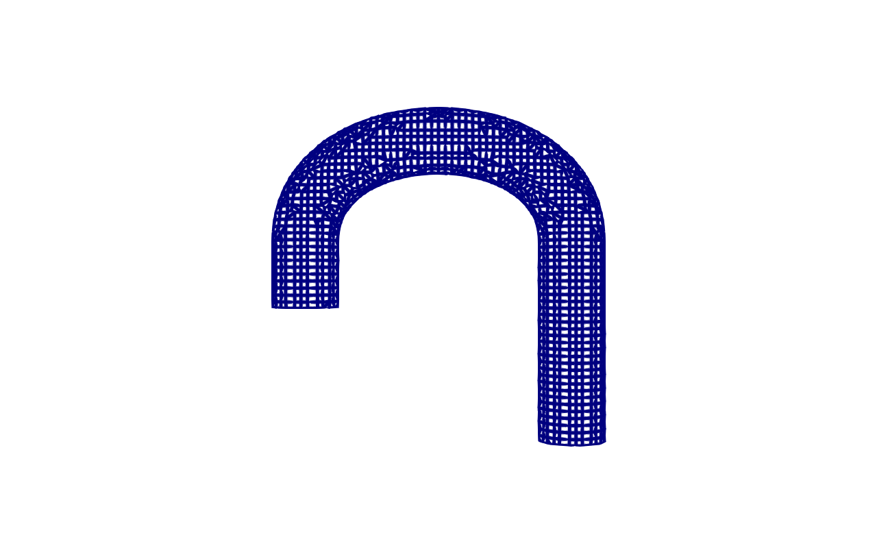 U-bend pipe mesh generated by snappyHexMesh. This tutorial teaches meshing and solver basics on a simple curved pipe before moving to patient-like geometries.
Hands-On Exercises
Mesh generation: exercise_01_mesh.tar.gz (52 KB) | ~10 sec | OpenFOAM 12
tar -xzf exercise_01_mesh.tar.gz && cd exercise_01_mesh
source /opt/openfoam12/etc/bashrc && ./run_mesh.sh
Solver comparison: exercise_05_solver.tar.gz (1.5 MB) | ~5 sec | OpenFOAM 12
Introduction
Before working with patient-specific aortic geometries, it is instructive to understand how AortaCFD generates meshes and drives the solver on a simple test case. This tutorial uses a U-bend pipe -- a curved tube with a single inlet and single outlet. The geometry is small enough that meshing completes in seconds and the solver finishes in under ten seconds, yet it exhibits curved-pipe flow physics (Dean vortices, asymmetric velocity profiles) that are directly relevant to aortic haemodynamics.
By the end of this tutorial you will be able to:
- Generate a volume mesh from an STL surface using snappyHexMesh.
- Read and interpret
checkMeshquality output. - Run the OpenFOAM solver with two different numerics profiles.
- Compare first-order (robust) and second-order (standard) solver behaviour.
- Identify healthy solver output in the log files.
Part 1: Mesh Generation
Extracting the Exercise
Download and extract the meshing exercise:
You will see the following contents:
| File | Purpose |
|---|---|
ubend.stl |
Surface geometry of the U-bend pipe (in millimetres) |
run_mesh.sh |
Shell script that executes the meshing pipeline |
system/blockMeshDict |
Background mesh definition |
system/snappyHexMeshDict |
Surface-conforming mesh parameters |
system/surfaceFeaturesDict |
Feature edge extraction settings |
Running the Meshing Pipeline
Source the OpenFOAM environment and run the mesh script:
The script executes three utilities in sequence:
- blockMesh creates a uniform hexahedral background mesh that encloses the STL geometry. This is the Cartesian starting grid.
- surfaceFeatures extracts sharp edges from the STL surface so that snappyHexMesh can preserve geometric features during snapping.
- snappyHexMesh carves the background mesh to conform to the STL surface in three stages: castellate (remove cells outside the geometry), snap (project cell vertices onto the surface), and optionally add boundary layers.
The entire process takes approximately 10 seconds on the U-bend geometry.
Understanding cells_per_diameter
The primary resolution control in AortaCFD is cells_per_diameter (cpd).
This parameter determines how many cells span the local vessel diameter. Drag the slider to explore:
| cpd | Approximate cell count (U-bend) | Use case |
|---|---|---|
| 8 | ~6,000 | Quick debugging |
| 10 | ~10,000 | Fast test |
| 12 | ~15,000 | Tutorial default |
| 15 | ~30,000 | Standard production |
| 20 | ~70,000 | Fine resolution |
For this exercise, cpd = 12 is used, producing approximately 15,000 cells. This is intentionally coarse -- sufficient for learning but not for publication-quality results.
How cpd Translates to Cell Size
AortaCFD reads the inlet diameter from the STL geometry and computes:
This cell size is then used to define the blockMeshDict grid spacing.
Increasing cpd by a factor of 2 increases cell count by approximately
a factor of 8 (cubic scaling in three dimensions).
Reading checkMesh Output
After snappyHexMesh completes, run checkMesh to assess mesh quality:
The output reports several quality metrics. The most important are:
Mesh non-orthogonality Max: 55.3 average: 8.7
Max skewness = 1.8 OK.
Max aspect ratio = 12.4 OK.
Mesh OK.
| Metric | Acceptable | Warning | Problematic |
|---|---|---|---|
| Max non-orthogonality | < 60 deg | 60--70 deg | > 70 deg |
| Max skewness | < 2 | 2--4 | > 8 |
| Max aspect ratio | < 50 | 50--100 | > 1000 |
Look for 'Mesh OK'
If checkMesh reports Mesh OK, the mesh passes all default quality
thresholds. If it reports warnings about non-orthogonality exceeding 70
degrees, the mesh may require refinement or the robust numerics profile
should be used.
Non-Orthogonality Above 70 Degrees
Meshes with non-orthogonality above 70 degrees can cause divergence with
second-order numerical schemes. If your mesh reports values in this range,
either increase cells_per_diameter to improve quality or use the
robust numerics profile, which tolerates poor mesh quality at the cost
of accuracy.
Part 2: Running the Solver
Extracting the Solver Exercise
Download and extract the solver exercise, which contains two pre-meshed U-bend cases:
| Directory | Numerics Profile | Schemes |
|---|---|---|
case_robust/ |
robust | Euler (time), upwind (convection) |
case_standard/ |
standard | backward (time), limitedLinearV (convection) |
Both cases use the same mesh, the same boundary conditions, and the same physical properties. The only difference is the numerical discretisation.
Running Both Cases
Each case completes in approximately 2--3 seconds.
foamRun vs Legacy Solvers
OpenFOAM 12 (Foundation version) uses the unified foamRun command with
the incompressibleFluid solver module, replacing the legacy
pimpleFoam solver. AortaCFD always targets foamRun.
Part 3: Comparing Profiles
Robust Profile (First Order)
The robust profile uses:
- Euler temporal discretisation -- first-order implicit, unconditionally stable, introduces temporal diffusion.
- upwind convection scheme -- first-order, maximum stability, smears velocity gradients.
This combination is extremely stable. It will run on virtually any mesh, including meshes with poor quality metrics. The trade-off is substantial numerical diffusion: velocity gradients near walls are artificially smoothed, causing wall shear stress to be systematically under-predicted.
Standard Profile (Second Order)
The standard profile uses:
- backward temporal discretisation -- second-order implicit, unconditionally stable, accurate phase resolution.
- limitedLinearV 1 convection scheme -- second-order TVD scheme, bounded, preserves sharp gradients while preventing non-physical overshoots.
This profile provides an appropriate balance between accuracy and stability for production cardiovascular CFD simulations. It requires reasonable mesh quality (non-orthogonality below approximately 65 degrees).
What to Look for in the Log
Examine the solver log for each case:
Key indicators of healthy solver behaviour:
| Indicator | Healthy | Unhealthy |
|---|---|---|
| Courant number max | < 1.0 | > 2.0 |
| PIMPLE convergence | Converged in 2--4 iterations | Not converged in 10 iterations |
| Pressure initial residual | Decreasing trend | Increasing or stagnant |
| Time step (deltaT) | Steady or slowly varying | Collapsing (< 1e-8) |
| Continuity error | < 1e-6 | > 1e-3 |
Time = 0.02s
Courant Number mean: 0.04 max: 0.87
PIMPLE: Iteration 1
  smoothSolver: Solving for Ux, Initial residual = 0.0012, Final residual = 8.3e-08
  GAMG:  Solving for p, Initial residual = 0.31, Final residual = 2.1e-06
PIMPLE: Converged in 3 iterations
Comparing Residuals Between Profiles
The robust profile typically shows lower residuals because the first-order schemes introduce more numerical diffusion, making the system easier to solve. Lower residuals do not mean higher accuracy -- they mean the numerical system is less demanding, which is a consequence of the additional artificial diffusion.
Physical Differences
If you visualise both results in ParaView, you will observe:
- Robust: smoother velocity field, rounded velocity profile at the bend, weaker secondary flow patterns.
- Standard: sharper velocity gradients, more pronounced Dean vortices in the bend, steeper near-wall velocity profiles.
The standard profile resolves flow features that the robust profile smears out. For clinical applications where wall shear stress matters, the standard profile is the minimum acceptable choice.
Summary
| Concept | Key Takeaway |
|---|---|
cells_per_diameter |
Primary mesh resolution control; cpd = 12 gives ~15K cells on U-bend |
checkMesh |
Always inspect non-orthogonality, skewness, and aspect ratio |
| Robust profile | 1st order (Euler + upwind); maximum stability, high diffusion |
| Standard profile | 2nd order (backward + limitedLinearV); accurate, needs good mesh |
| Solver log | Monitor Courant number, PIMPLE convergence, and residual trends |
| Mesh quality vs profile | Higher-order schemes demand better mesh quality |
What's Next
In Tutorial 2: Inlet and Outlet Conditions, you will learn how AortaCFD handles physiological boundary conditions -- pulsatile inlet flow waveforms and Windkessel outlet models that represent the downstream vasculature.
References
Full bibliography on the References page.
Found an issue or have a suggestion for this page?
Open a GitHub issue