Tutorial 3: Synthetic Aorta Pipeline

Goal: Run the complete AortaCFD pipeline on a patient-like synthetic geometry -- an aortic arch with coarctation and three supra-aortic branches.

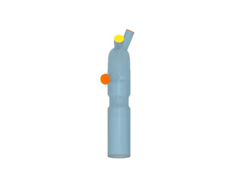
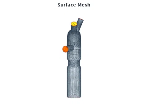
Geometry: arch + branches + coarctation	Mesh: surface → cross-section (200K cells)

Hands-On Exercise

Download: exercise_g3_quick.tar.gz (523 KB) | ~30 sec | OpenFOAM 12

Synthetic aortic arch (G3) with 65% coarctation. Complete pipeline from STL to solution.

tar -xzf exercise_g3_quick.tar.gz && cd exercise_g3_quick
source /opt/openfoam12/etc/bashrc
./run.sh

---

Introduction

The previous tutorials introduced meshing and boundary conditions on simple tube geometries. This tutorial brings those concepts together on a patient-like aortic arch -- a synthetic geometry generated by the Blender parametric tool in this project. The G3 geometry includes an aortic arch with three supra-aortic branches and a 65% coarctation (area reduction at the aortic isthmus), making it a clinically relevant benchmark.

Synthetic geometries serve an essential role in computational haemodynamics research:

• Controlled parameters: The coarctation severity, branch angles, and vessel diameters are known exactly, enabling systematic parametric studies.
• Reproducibility: Any researcher can regenerate the identical geometry from the Blender script, eliminating segmentation variability.
• Ground truth: Because the geometry is analytically defined, mesh convergence studies and code verification are straightforward.
• No ethics approval required: Synthetic cases can be shared freely as teaching and benchmarking material.

By the end of this tutorial you will be able to:

1. Identify the STL patches and their anatomical correspondence.
2. Read and interpret an AortaCFD configuration file.
3. Run the full pipeline (mesh generation through solver execution).
4. Examine the output directory structure and verify mesh quality.
5. Understand the haemodynamic significance of aortic coarctation.

---

The G3 Geometry

The G3 synthetic aortic arch has the following specifications:

Feature	Value
Main aortic diameter	24 mm
Coarctation severity	65% area reduction
Coarctation location	Aortic isthmus (distal to left subclavian)
Supra-aortic branches	3 (brachiocephalic, LCCA, LSA)
Outlets	4 (3 branches + descending aorta)
STL units	Millimetres

The coarctation creates a geometric narrowing at the isthmus -- the segment of the aorta just distal to the left subclavian artery origin. Clinically, coarctation of the aorta is a congenital condition that produces a trans-stenotic pressure gradient and accelerated flow through the narrowing. The ESC guidelines define a resting pressure gradient exceeding 20 mmHg as the threshold for intervention Erbel 2014.

Anatomical Orientation

The aortic arch curves from the ascending aorta (rising from the left ventricle) over the pulmonary trunk and descends as the thoracic aorta. Three branches arise from the superior aspect of the arch:

1. Brachiocephalic trunk (innominate artery) -- supplies the right arm and right side of the head.
2. Left common carotid artery (LCCA) -- supplies the left side of the head.
3. Left subclavian artery (LSA) -- supplies the left arm.

---

Case Input Structure

Extract the exercise and examine the contents:

tar -xzf exercise_g3_quick.tar.gz
cd exercise_g3_quick
ls

The input directory contains the following files:

File	Purpose	Anatomical Correspondence
inlet.stl	Inlet patch surface	Ascending aorta (flow enters here)
outlet1.stl	Outlet patch 1	Brachiocephalic trunk
outlet2.stl	Outlet patch 2	Left common carotid artery
outlet3.stl	Outlet patch 3	Left subclavian artery
outlet4.stl	Outlet patch 4	Descending aorta
wall_aorta.stl	Wall patch surface	Aortic wall (WSS computed here)
config.json	Simulation configuration	All pipeline parameters

Each STL file represents one boundary patch of the simulation domain. The patches must be watertight (no gaps between adjacent patches) and oriented with outward-facing normals. AortaCFD reads the inlet diameter from inlet.stl to determine the mesh resolution.

STL Naming Convention

AortaCFD identifies patches by filename: inlet.stl is always the inlet, files matching outlet*.stl are outlets, and wall_aorta.stl is the vessel wall. This convention must be followed for the pipeline to assign boundary conditions correctly.

---

Understanding the Config

Open the configuration file:

cat config.json

The configuration is organised into sections. The quick tutorial config uses deliberately simplified settings for fast execution:

case_info

{
  "case_info": {
    "case_name": "G3",
    "description": "Synthetic aortic arch with 65% coarctation"
  }
}

Identifies the case. The case_name is used to create the output directory.

physics

{
  "physics": {
    "model": "laminar",
    "density": 1060,
    "dynamic_viscosity": 0.004
  }
}

Parameter	Value	Notes
model	laminar	No turbulence model; appropriate for Re < 4000
density	1060 kg/m^3	Standard blood density
dynamic_viscosity	0.004 Pa.s	Newtonian blood assumption

Kinematic Viscosity

OpenFOAM internally uses kinematic viscosity: \(\nu = \mu / \rho = 0.004 / 1060 = 3.774 \times 10^{-6}\) m^2/s. AortaCFD performs this conversion automatically.

numerics

{
  "numerics": {
    "profile": "robust"
  }
}

The quick config uses the robust profile (first-order schemes) for maximum stability on the coarse mesh. For production simulations, switch to standard.

mesh

{
  "mesh": {
    "cells_per_diameter": 10,
    "boundary_layers": {
      "enabled": false
    }
  }
}

Parameter	Value	Notes
cells_per_diameter	10	Coarse; produces ~50,000--100,000 cells
boundary_layers	disabled	No prismatic layers; WSS will be approximate

Boundary Layers Disabled

This quick config intentionally disables boundary layers to reduce meshing time. Wall shear stress computed without boundary layers is unreliable. For any study reporting WSS metrics, enable boundary layers with at least 3--5 prismatic layers.

geometry

{
  "geometry": {
    "scale_factor": 0.001,
    "keywords": ["aorta", "coarctation"]
  }
}

The scale_factor of 0.001 converts STL coordinates from millimetres to metres (OpenFOAM's internal unit system). This is a critical parameter -- an incorrect scale factor is one of the most common sources of error in cardiovascular CFD.

Always Verify the Scale Factor

If the STL is already in metres, set scale_factor to 1.0. If it is in millimetres (as is standard for medical imaging STL exports), use 0.001. A wrong scale factor produces a domain 1000x too large or too small, leading to nonsensical velocities and pressures. Check the inlet audit report after case setup to verify the inlet area is physiologically reasonable (~3--5 cm^2 for an adult aorta).

boundary_conditions

{
  "boundary_conditions": {
    "inlet": {
      "type": "CONSTANT",
      "cardiac_output": 5.0,
      "profile": "plug"
    },
    "outlets": {
      "type": "zeroGradient"
    }
  }
}

The quick config uses the simplest boundary conditions: constant inlet flow and zeroGradient outlets. This is sufficient for verifying that the mesh and solver work correctly. For physiological results, use TIMEVARYING inlet and 3EWINDKESSEL outlets as described in Tutorial 2.

simulation_control

{
  "simulation_control": {
    "end_time": 0.05,
    "parallel": false,
    "num_processors": 1
  }
}

Parameter	Value	Notes
end_time	0.05 s	Very short; just enough to see the flow develop
parallel	false	Serial execution; no domain decomposition
num_processors	1	Single core

Production Settings

A full cardiac cycle simulation (3 cycles at 0.8 s each = 2.4 s) with Windkessel outlets, cpd = 15, boundary layers, and 8 processors is a typical production configuration. The quick config here runs in ~30 seconds to demonstrate the pipeline workflow.

---

Running the Pipeline

There are two ways to execute the simulation.

Option A: Using AortaCFD (Recommended)

If you have AortaCFD cloned and its virtual environment set up:

source /opt/openfoam12/etc/bashrc
cd /path/to/AortaCFD
source venv/bin/activate

python run_patient.py G3 \
    --config /path/to/exercise_g3_quick/config.json \
    --run-name tutorial \
    --steps case,mesh,boundary,solver

AortaCFD orchestrates the complete pipeline:

1. case -- Creates the OpenFOAM directory structure, copies STL files, renders Jinja2 templates for all dictionaries.
2. mesh -- Runs blockMesh, surfaceFeatures, snappyHexMesh, and checkMesh.
3. boundary -- Generates the 0/U and 0/p boundary condition files from the configuration.
4. solver -- Executes foamRun (or mpirun -np N foamRun for parallel cases).

Option B: Manual OpenFOAM Steps

If you prefer to run the OpenFOAM utilities directly (useful for learning what AortaCFD automates):

source /opt/openfoam12/etc/bashrc
cd exercise_g3_quick

# 1. Generate background mesh
blockMesh

# 2. Extract surface features
surfaceFeatures

# 3. Generate volume mesh (castellate, snap, layers)
snappyHexMesh -overwrite

# 4. Check mesh quality
checkMesh

# 5. Run the solver
foamRun

The -overwrite Flag

By default, snappyHexMesh writes each stage to a separate time directory (1/, 2/, 3/). The -overwrite flag writes the final mesh directly to constant/polyMesh/, which is the expected location for subsequent utilities and the solver.

Using the Provided run.sh Script

The exercise includes a convenience script:

./run.sh

This script sources the OpenFOAM environment, runs all meshing steps, checks the mesh, and starts the solver. It is equivalent to Option B above.

---

Examining the Output

Mesh Quality

After meshing, inspect the checkMesh output:

checkMesh | tail -20

Expected output for cpd = 10 on the G3 geometry:

Checking geometry...
    Overall domain bounding box (-0.015 -0.06 -0.015) (0.015 0.005 0.04)
    Mesh has 3 geometric (non-empty/wedge) directions (1 1 1)
    Mesh has 3 solution (non-empty) directions (1 1 1)

Checking topology...
    Cell to face addressing OK.
    Point usage OK.

Checking geometry...
    Max non-orthogonality = 58.2 OK.
    Max skewness = 2.1 OK.
    Max aspect ratio = 18.7 OK.

Mesh OK.

Cell Count

With cpd = 10 and no boundary layers, expect approximately 50,000 to 100,000 cells. The exact count depends on the snappyHexMesh refinement algorithm's interaction with the geometry. Check the checkMesh output for the line reporting cells:.

Solution Fields

After the solver completes, time directories appear in the case:

ls -d 0.0*

Each time directory contains the velocity (U) and pressure (p) fields. Open the final time step in ParaView:

paraview exercise_g3_quick.foam &

1. Click Apply to load the mesh.
2. Set representation to Surface.
3. Colour by U (velocity magnitude) -- observe the flow acceleration through the coarctation.
4. Colour by p (pressure) -- observe the pressure drop across the narrowing.

Key Flow Features

On the G3 geometry with 65% coarctation, you should observe:

Feature	Location	Physical Significance
Accelerated jet	Through the coarctation	Continuity: reduced area forces higher velocity
Pressure drop	Across the coarctation	Energy loss due to acceleration and viscous dissipation
Recirculation zone	Distal to the coarctation	Flow separation from the expansion
Branch flow	Supra-aortic arteries	Flow diverted to head and arms

The Coarctation Jet

The 65% area reduction forces the blood to accelerate through the narrowing. By the continuity equation, if the area is reduced by 65%, the velocity increases by a factor of approximately 2.9. This high-velocity jet impinges on the distal wall, creating elevated wall shear stress, and the sudden expansion downstream produces a recirculation zone with disturbed flow. These are the primary haemodynamic features of aortic coarctation that guide clinical intervention decisions.

---

Exercise: Modify the Config and Re-Run

1. Copy the configuration file:

   cp config.json config_standard.json
   

2. Edit config_standard.json to change:

   • numerics.profile from "robust" to "standard"
   • mesh.cells_per_diameter from 10 to 15
   • mesh.boundary_layers.enabled from false to true

3. Re-run the pipeline with the updated config.

4. Compare the two results:

   • How does the cell count change?
   • Is the checkMesh quality different?
   • Are the velocity gradients near the coarctation sharper with the standard profile?

Expected Differences

Increasing cpd from 10 to 15 approximately doubles the cell count (cubic scaling). Enabling boundary layers adds prismatic cells near the wall, improving WSS resolution. The standard profile resolves sharper velocity gradients through the coarctation compared to the robust profile.

---

Summary

Concept	Key Takeaway
Synthetic geometry	Controlled, reproducible, known ground truth; ideal for benchmarking
G3 coarctation	65% area reduction at the isthmus; creates pressure gradient and jet
STL patches	inlet, outlet1--4, wall_aorta; named by convention for AortaCFD
scale_factor	0.001 converts mm to m; verify via inlet area in audit report
Quick config	cpd = 10, robust, no layers, constant inlet, 0.05 s; ~30 seconds
Pipeline steps	case, mesh, boundary, solver; can run individually or together
Output	Time directories with U and p fields; checkMesh for quality

---

What's Next

In Tutorial 4: Hemodynamics and Post-Processing, you will use pre-computed pulsatile results on this same G3 geometry to compute and interpret clinically relevant haemodynamic metrics: TAWSS, OSI, RRT, and trans-coarctation pressure gradient.

---

References

Full bibliography on the References page.

Found an issue or have a suggestion for this page?

Open a GitHub issue