Tutorial 5: Real Patient Case
Goal: Run a complete simulation on a real patient-specific aortic geometry.
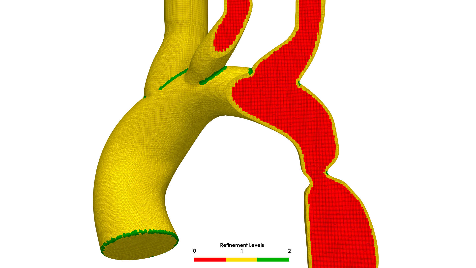 BPM120: real paediatric aortic coarctation geometry. 4.8M cell mesh with boundary layers generated by AortaCFD's snappyHexMesh pipeline.
Case
Geometry: BPM120 --- published paediatric aortic coarctation (Wang et al.) Runtime: ~30 seconds (quick), ~2 minutes (pulsatile coarse), ~30 minutes (production) Requires: AortaCFD installed, OpenFOAM 12, Python venv activated
Prerequisites
- Completed Tutorials 1--4 (mesh generation, boundary conditions, solver, hemodynamics)
- AortaCFD repository cloned and Python virtual environment activated
- OpenFOAM 12 sourced (
source /opt/openfoam12/etc/bashrc) - Windkessel boundary condition library compiled (see Getting Started)
Learning Objectives
By the end of this tutorial you will be able to:
- Run the complete AortaCFD pipeline on a real patient geometry.
- Distinguish between quick-test, coarse-pulsatile, and production configurations.
- Interpret the output directory structure and provenance files.
- Compare results between different numerics profiles.
- Execute batch processing for multi-case cohort studies.
The BPM120 Case
BPM120 is a published paediatric aortic coarctation case used as the primary test geometry throughout the AortaCFD documentation. Key characteristics:
| Property | Value |
|---|---|
| Anatomy | Paediatric thoracic aorta with coarctation |
| Heart rate | 120 BPM (cardiac period 0.5 s) |
| Outlets | 4 (brachiocephalic trunk, left common carotid, left subclavian, descending aorta) |
| Geometry source | Segmented from contrast-enhanced CT angiography |
| STL units | Millimetres (scale factor 0.001) |
The case directory contains multiple configuration files at different fidelity levels:
cases_input/BPM120/
├── inlet.stl
├── outlet1.stl
├── outlet2.stl
├── outlet3.stl
├── outlet4.stl
├── wall_aorta.stl
├── flowrate.csv
├── config.json                    # Production (full fidelity)
├── config_tutorial_simple.json    # Fastest: constant inlet, zeroGradient outlets
└── config_tutorial_coarse.json    # Intermediate: pulsatile, Windkessel, coarse mesh
Quick First Run
The fastest way to verify that the pipeline works is the --quick flag, which internally uses a simplified configuration (constant inlet, zeroGradient outlet boundary conditions, coarse mesh, robust numerics profile, 0.1 s simulation time):
source /opt/openfoam12/etc/bashrc
cd /path/to/AortaCFD

python run_patient.py BPM120 --quick --run-name first_test
What --quick Does
The --quick flag is a convenience shortcut that applies config_tutorial_simple.json internally. It produces a coarse, steady-state approximation suitable for verifying that the geometry meshes correctly and the solver runs to completion. It is not suitable for hemodynamic analysis.
Expected behaviour:
- Meshing: ~20 seconds, producing approximately 200k--400k cells
- Solver: ~10 seconds, 0.1 s of simulated time with constant inlet velocity
- Total wall time: approximately 30 seconds
Inspect the output:
The output directory contains:
| Directory | Contents |
|---|---|
openfoam/ |
Complete OpenFOAM case (0/, constant/, system/, time directories) |
reports/ |
merged_config.json, simulation_setup_report.txt, hemodynamics_report.txt |
results/ |
qoi_summary.json, qoi_summary.csv |
Pulsatile Run
For a physiologically meaningful simulation, use the coarse tutorial configuration, which includes a pulsatile inlet waveform, Windkessel outlet boundary conditions, and one complete cardiac cycle:
This configuration runs in approximately 2 minutes on a modern workstation and produces results suitable for initial hemodynamic assessment. The key differences from the quick run:
| Parameter | Quick (--quick) |
Pulsatile Coarse | Production (config.json) |
|---|---|---|---|
| Inlet type | CONSTANT | TIMEVARYING (CSV) | TIMEVARYING (CSV) |
| Inlet profile | plug | parabolic | wall_distance |
| Outlet BCs | zeroGradient | 3EWINDKESSEL | 3EWINDKESSEL |
| Numerics profile | robust | robust | standard |
| Mesh (cells/D) | 8 | 10 | 15 |
| Simulation time | 0.1 s | 0.5 s (1 cycle) | 1.5 s (3 cycles) |
| Parallel | serial | serial | 4 cores |
| Approximate runtime | ~30 s | ~2 min | ~30 min |
| Suitable for | Pipeline verification | Initial assessment | Publication |
Understanding the Configuration Variants
config_tutorial_simple.json
The simplest configuration. Uses a constant inlet velocity derived from cardiac output, zeroGradient outlets (fixed zero pressure), and the robust numerics profile. No pulsatility, no Windkessel coupling. The purpose is exclusively to verify that the geometry meshes correctly and the solver runs without crashing.
config_tutorial_coarse.json
Introduces physiological boundary conditions: a pulsatile flow waveform from flowrate.csv and three-element Windkessel outlets calibrated from blood pressure (120/80 mmHg). The mesh is coarse (10 cells per inlet diameter) and the numerics profile is robust (first-order schemes). This produces qualitatively correct hemodynamic patterns at low computational cost.
config.json (Production)
Full-fidelity configuration for publication-quality results. Uses the standard numerics profile (second-order temporal and spatial discretisation), finer mesh (15 cells per inlet diameter), wall-distance inlet profile, and three cardiac cycles with analysis on the final cycle. Requires parallel execution on 4 or more cores.
Start Coarse, Refine Later
For any new patient geometry, always begin with config_tutorial_simple.json to verify that the pipeline completes without errors. Then progress to config_tutorial_coarse.json for initial hemodynamic assessment. Only run the full production configuration once the coarse results are satisfactory.
Examining Results
Output Directory Structure
output/BPM120/pulsatile_test/
├── openfoam/
│   ├── 0/                    # Initial and boundary conditions
│   ├── constant/             # Mesh and physical properties
│   ├── system/               # Solver controls
│   ├── 0.01/, 0.02/, ...    # Solution snapshots
│   └── logs/                 # Solver and mesh log files
├── reports/
│   ├── merged_config.json    # Fully resolved configuration (provenance)
│   ├── simulation_setup_report.txt
│   ├── hemodynamics_report.txt
│   └── inlet_audit.json
└── results/
    ├── qoi_summary.json      # Structured QoI data
    └── qoi_summary.csv       # Tabular QoI data
Provenance: merged_config.json
The merged_config.json file captures the fully resolved configuration after the three-layer merge (base defaults + numerics profile + case JSON). This file is sufficient to reproduce any simulation exactly:
Reproducibility
Include merged_config.json as supplementary material in publications. Another researcher with the same STL files and AortaCFD version can reproduce the simulation exactly from this file.
QoI Summary
Compare the hemodynamic metrics against the clinical thresholds from Tutorial 4:
- Is the pressure drop below 20 mmHg?
- Is the mean TAWSS within the normal range (1--3 Pa)?
- Are there regions of elevated OSI (> 0.2)?
Profile Comparison
A valuable verification exercise is to run the same case with different numerics profiles and compare the results. The robust profile uses first-order schemes that introduce numerical diffusion; the standard profile uses second-order schemes with minimal diffusion.
# Robust profile (first-order, maximum stability)
python run_patient.py BPM120 \
    --config config_tutorial_coarse.json \
    --profile robust \
    --run-name profile_robust

# Standard profile (second-order, higher accuracy)
python run_patient.py BPM120 \
    --config config_tutorial_coarse.json \
    --profile standard \
    --run-name profile_standard
Compare the QoI summaries:
cat output/BPM120/profile_robust/results/qoi_summary.json
cat output/BPM120/profile_standard/results/qoi_summary.json
Expected observations:
| Metric | Robust vs Standard |
|---|---|
| Pressure drop | Similar (within 5--10%); pressure is a global metric insensitive to numerical diffusion |
| TAWSS P95 | Standard typically 10--30% higher; first-order diffusion smears near-wall gradients |
| OSI | Standard typically higher; oscillatory features are damped by first-order schemes |
Profile Sensitivity
If TAWSS P95 differs by more than 30% between robust and standard profiles, the mesh is likely too coarse. Increase cells_per_diameter and re-run the comparison. On an adequately resolved mesh, the profile difference should be modest.
Batch Execution
For cohort studies involving multiple patient geometries, the run_batch.py script provides parallel execution:
| Flag | Purpose |
|---|---|
--cases |
Specify which patient cases to process |
--workers |
Number of parallel simulation workers |
--config-list |
Run different configurations for the same or different geometries |
Upon completion, batch processing generates a cohort_comparison.csv file aggregating QoI values from all completed simulations into a single table suitable for statistical analysis.
Resource Management
Each OpenFOAM simulation is memory-intensive. When setting --workers, ensure that the total memory consumption does not exceed available RAM. A single aortic simulation with 2M cells typically requires 4--8 GB of memory.
Exercise 1: Three-Stage Progression
Run the BPM120 case at all three fidelity levels and compare:
python run_patient.py BPM120 --quick --run-name ex_quickpython run_patient.py BPM120 --config config_tutorial_coarse.json --run-name ex_coarsepython run_patient.py BPM120 --run-name ex_production(if time permits)
For each run, record:
| Run | Cell count | Runtime | Pressure drop (mmHg) | TAWSS P95 (Pa) |
|---|---|---|---|---|
| Quick | ||||
| Coarse pulsatile | ||||
| Production |
How do the hemodynamic metrics change with increasing fidelity?
Exercise 2: Profile Comparison
Run the coarse pulsatile configuration with both robust and standard profiles (as described above). Compare:
- Pressure drop: is the difference within 10%?
- TAWSS P95: how much higher is the standard-profile value?
- Open both results in ParaView and compare the WSS distribution visually.
Discussion
Which hemodynamic metrics are sensitive to the numerics profile, and which are robust? What does this tell you about the relative importance of mesh resolution versus numerical scheme selection?
What's Next
Tutorial 6 covers publication-quality verification studies: mesh convergence with GCI analysis, Large Eddy Simulation for transitional flow, and automated methods-paragraph generation for manuscripts.
References
Full bibliography on the References page.
Found an issue or have a suggestion for this page?
Open a GitHub issue